The graph that lets AI write code without breaking things
When an AI agent is editing a codebase, the question it has to answer before every change is the same one a careful human asks: what else will this break? A naive AI sees the function it’s editing. A grounded AI sees the call graph, the import chain, the inheritance tree — every place that function is referenced from, every caller that depends on its current signature, every test that might fail. The difference between “the AI proposes a fix” and “the AI proposes a fix that ships without regressing six other things” is whether it has access to that structural ground truth, or has to guess from the file it can see.
This is exactly the problem Google’s Kythe and GitHub’s CodeQL were built to solve for human developers — semantic indexing of source code as a graph, queryable for cross-references, dependencies, and structural relationships. Kythe is Google’s open-source ecosystem for code-analysis tooling — the public effort to provide the kind of code-as-graph primitives their internal tooling has long relied on. CodeQL powers GitHub’s security scanning. The same shape, applied to LLM-driven development, is what this platform needed: a program dependency graph, queryable through MCP tools, so the AI doing the editing has the same map of the codebase that an experienced human holds in their head.
I asked Claude to research how this is done at scale. The output pointed at two patterns worth lifting. The first is demand-driven graph navigation — build the graph once, then let queries walk it (RepoAudit, arXiv:2501.18160 reports 78.43% precision on real bugs using exactly this shape). The second is end-to-end journey tracing — once you have the graph, BFS from any entry point recovers the actual execution flow, which is the thing an AI most often needs when it asks “what does this code path actually do end-to-end?”. Both became MCP tools (analyze_code_impact, get_processes) the agent can call mid-task without leaving the conversation.
S3E1 shipped the Code Knowledge Graph’s infrastructure — the PDG generator, the FalkorDB instance, the D3.js force-directed viewer on NodePort 30650. S3E4 reported the code_intelligence graph at around 2,000 nodes from an early build. Both episodes were accurate at the time. Neither described a graph that was stable: earlier populate runs had been partial-scope, or in-memory and never exported, or exported and not persisted across pod restarts. The wiring was in place since January; the data behind it kept evaporating.
The arc across the season looks like this:
S3E1 S3E4 THIS EPISODE Today
(Jan 25) (Feb 21) (Mar 8–19) (May)
──────── ──────── ──────────── ───────
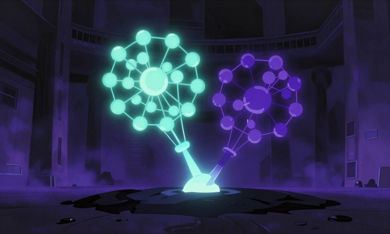
PDG code ~2,000 nodes 12,985 nodes, stable + dependable
+ FalkorDB from an early 16,137 edges, queryable end-to-end
+ D3.js partial build Leiden clustering by AI agents:
viewer ships that didn't activated, 312 communities,
survive a Scout Fleet shipped, 162 execution flows
redeploy NER reversal landedThis is the eleven days where the second graph stopped being intermittent and became dependable — the first full-codebase populate that took, plus the layers that made the graph more than a static lookup table. It runs from March 8th to March 19th. Four architectural decisions made it work: an AST-only graph builder for portability, Leiden clustering to surface emergent community structure, a two-topic Kafka pipeline with graceful-degradation semantics, and a deliberate reversal from LLM-based to deterministic NLP that cut hallucinated tags from 75% to 0.3%. The decisions are in service of one goal — make AI-driven development reliable enough that the AI doesn’t break code it touches — by making the structural shape of the codebase a thing the AI can query reliably, not a thing it has to guess at when the graph happens to be populated.
If you only read one section of what follows, read the one on the NER reversal. We tried to use a 14-billion-parameter language model to do span-based entity extraction; it hallucinated 75% of its output by fabricating entities from prompt context that did not appear in the source document. We replaced it with spaCy’s en_core_web_lg plus rule-based patterns plus a statistical keyword extractor, and precision went from 25% to 99.7% in a single deploy. That gap exists because we picked the wrong tool for the problem class — exactly the kind of trap an AI agent walks into when it has no structural ground truth to fall back on. The architectural lesson generalises further than NER.

Where the system stood (March 2026)
This was the platform at the start of the episode. The L4 inference layer was still serving Qwen3-14B-AWQ (Qwen3-8B-AWQ doesn’t land until May — that’s a later episode about smoke gates and thinking-mode leaks). The journal streaming pipeline from S3E2 was running. The Matrix bot from S3E4 was producing real answers. The vault sat at around 4K documents in Qdrant (148K chunks after embedding).
┌─────────────────────────────────────────────────────────────┐
│  L1 PRESENTATION                                            │
│  Obsidian · LibreChat · Grafana · Element/Matrix            │
└─────────────────────────────────────────────────────────────┘
                            │
┌─────────────────────────────────────────────────────────────┐
│  L2 SERVICE GATEWAYS                                        │
│  MCP Bridge :30002 (22 tools)  ·  RAG Gateway :30808        │
└─────────────────────────────────────────────────────────────┘
                            │
┌─────────────────────────────────────────────────────────────┐
│  L3 AGENTS                                                  │
│  FastSearchAgent · DeepResearchAgent · AgentRouter          │
│  (no OracleAgent yet — that lands later)                    │
└─────────────────────────────────────────────────────────────┘
                            │
┌─────────────────────────────────────────────────────────────┐
│  L4 INFERENCE                                               │
│  vLLM Qwen3-14B-AWQ · TEI Embedding · FlashRank             │
└─────────────────────────────────────────────────────────────┘
                            │
┌─────────────────────────────────────────────────────────────┐
│  L5 DATA  ← THIS POST                                       │
│                                                             │
│   Qdrant ~4K docs (148K chunks) · BM25 hybrid               │
│   (server-side RRF comes in a later episode)                │
│                                                             │
│   FalkorDB:                                                 │
│     document_knowledge      ← was there before (S3E4)       │
│     code_knowledge          ← NEW THIS EPISODE              │
│                                                             │
│   Kafka topics (existing): journal.*                        │
│   Kafka topics (NEW):      vault.file-events                │
│                            vault.file-tagged                │
└─────────────────────────────────────────────────────────────┘
The headline change is the code-knowledge graph going from a design in an ADR to 12,985 nodes and 16,137 edges in a live FalkorDB instance. The supporting change is two new Kafka topics that decouple entity extraction from embedding, and a separate consumer for each.
The four decisions that shape the rest of the episode all sit at L5, the data layer.
Decision 1: AST-only Pipeline 1, defer the LLM-augmented graph
This wasn’t a from-scratch build. By the morning of March 10th, four foundation tickets had already shipped: VW-79 integrated Graphiti and FalkorDB as the platform’s graph backbone, declaring both document_knowledge and code_intelligence in a single FalkorDB instance. VW-100 registered the seven PDG MCP tools into the production bridge — analyze_code_impact, get_dependency_graph, the works — and wired the journey tracer. VW-102 unlocked the full tool surface including the FalkorDB sync and Confluence integration. VW-104 fixed Cypher dialect incompatibilities that had been tripping up early queries. All four Done. And the D3.js frontend on NodePort 30650 from S3E1 had been serving the visualisation since January.
And yet, on the morning of March 10th, the FalkorDB code_intelligence graph wasn’t reliably populated. S3E4’s ~2,000-node figure had come from a partial-scope build that hadn’t survived a redeploy; subsequent populate attempts ran in memory and weren’t exported, or exported but didn’t persist across pod restarts. The wiring was in place. The data behind it kept evaporating. An MCP agent calling analyze_code_impact on a Monday could get useful results; by Friday the same call would return an empty response.
This episode is the activation step where the populate-and-persist cycle finally took. The PDG (Program Dependency Graph) generator had been designed with two pipelines: Pipeline 1 walks Python AST and extracts modules, classes, functions, methods, calls, imports, and inheritance — pure static analysis, no model required. Pipeline 2 would use an LLM to extract semantic relationships that AST can’t see — “this function is a retry decorator”, “this class implements the Strategy pattern”, “these two modules communicate through a shared global”. Pipeline 2 is richer. Pipeline 1 is cheaper.
I activated Pipeline 1 alone and explicitly deferred Pipeline 2.
The trade-off table:
| Approach | Trade-off | Verdict |
|---|---|---|
| Activate Pipeline 1 only | A less semantically rich graph. The structural edges (CALLS, INHERITS, IMPORTS, CONTAINS) are there. The semantic annotations aren’t. Zero LLM dependency means the graph is buildable on any machine with Python, no GPU required, no inference service required. | Chosen. |
| Activate Pipeline 1 and Pipeline 2 together | Richer graph at first deploy. But every rebuild requires vLLM to be available. The cluster has one GPU; vLLM is shared between the LLM serving and the embedding model. Coupling the code graph to GPU availability means rebuilds queue behind whoever else needs the hardware. | Rejected — adds a dependency that doesn’t have to be there. |
| Defer the code graph entirely until Pipeline 2 is ready | Wait for the better thing. But the AST graph is already useful for the questions I want answered: “if I change rootweaver-core/config.py, what else breaks?”, “which modules depend on the gateway?”, “what’s the blast radius of a function rename?” Those are answerable without any LLM. | Rejected — the existing AST data answers most of the actual questions. |
The first run on the platform codebase produced 12,985 nodes and 16,137 edges in 352.9 seconds. That’s 1,128 Python files parsed across 40,057 candidate files (the rest excluded — virtualenvs, .worktrees/, __pycache__). The breakdown:
| Node type | Count | What it represents |
|---|---|---|
| Method | 6,082 | Bound functions on classes |
| Function | 2,829 | Module-level functions |
| Class | 1,550 | Type definitions |
| Variable | 1,404 | Module-level globals |
| Module | 1,128 | Python files |
Edge counts: CONTAINS dominates at 73.5% (a module contains a class contains methods), CALLS is 18.0%, IMPORTS is 8.1%, INHERITS is the long tail at 0.4%. That distribution alone is informative — it tells you the codebase is more functional than object-oriented, and that inheritance is rarer than I’d assumed.
But raw nodes and edges aren’t what makes the graph useful to an AI. The interface is. Seven MCP tools went live with the graph, each one a different question an agent can ask without reading any source code:
| MCP tool | Question it answers | Typical response size |
|---|---|---|
analyze_code_impact | If I change this file, what else breaks? | ~105 tokens |
find_module_dependents | Who imports this module? | ~102 tokens |
get_dependency_graph | Show me the module dependency tree at depth N | ~2,100 tokens |
search_modules | Find modules whose name or path matches X | ~190 tokens |
detect_tags_in_file | What tags does this file declare? | ~50 tokens |
get_pdg_stats | Is the graph healthy and how big is it? | ~85 tokens |
rebuild_pdg | Refresh the graph after a code change | n/a |
These are the seams the AI calls across when it needs structural ground truth. Before this activation, an agent asked to refactor a function would either guess at the blast radius or grep the codebase manually — both error-prone, the second slow. After this activation, an agent could call analyze_code_impact(["rootweaver-core/config.py"]) and get back a structured ImpactReport — affected modules, recommendations, a risk score — in about 105 tokens. The AI doesn’t have to read the codebase. The graph already did.
The architectural lesson generalises. When you have two pipelines and one is portable and the other requires bespoke infrastructure, ship the portable one first. The richer pipeline can come later as an opt-in. Some of this code might one day run in other enterprise environments where you can’t assume a GPU or an LLM endpoint exists — and the AST-only path means the graph is reproducible there without modification. Defer the dependency until it’s earned.
Decision 2: Leiden clustering for emergent community structure
A graph with 12,985 nodes is searchable but not browsable. You can ask “show me everything that depends on the gateway” and get back a Mermaid diagram, but you can’t ask “what are the natural functional clusters in this codebase?” because that requires the algorithm to discover them, not for you to enumerate them.
The decision was: don’t try to enumerate the architecture by hand. Run a community detection algorithm and let it surface the clusters.
I used the Leiden algorithm (Traag, Waltman, van Eck, Scientific Reports 2019) via python-igraph. Leiden is a refinement of Louvain that guarantees well-connected communities — it doesn’t produce the badly-connected clusters that Louvain can occasionally leave behind. For a code graph where the question is “which nodes belong together”, that guarantee matters: a well-connected community is a real cluster, not an artifact of the algorithm’s random walk.
Edge weights drive what Leiden treats as “belonging together”. I chose them deliberately:
| Edge type | Weight | Reasoning |
|---|---|---|
| CALLS | 3.0 | The strongest coupling signal. Functions that call each other usually share purpose. |
| INHERITS | 2.0 | Subclasses and parents are tightly bound but not always frequently exercised together. |
| IMPORTS | 1.0 | Common-utility imports are weak signals — every module imports os and logging but those imports don’t mean the modules are related. |
Production run produced 252 communities and 140 execution flows, where an execution flow is a BFS-traced call chain from an entry point that runs at least 3 steps deep. The top community contains 148 members and corresponds to the platform’s RAG innovations and experimental layer. The community containing AgentRouter and BatchIndex is 91 members — that’s the RAG production core (gateway, agents, retriever) discovered automatically.
This is the part I didn’t expect. The communities don’t match the directory structure. They cut across packages. Code that belongs together by call-graph analysis isn’t always code that lives in the same folder. The algorithm reveals an organisational truth the file system hides.
The trade-off is interpretability. Manual taxonomies have meaningful names. Algorithmic communities have IDs. To make them human-readable I added a vLLM labelling step gated behind an environment variable (PDG_VLLM_LABELS=true) — when enabled, the platform’s LLM generates a label for each community from its top members. So community 17 becomes Alert_and_Context_Management instead of cluster_17. When the flag is off, the algorithmic IDs persist. The labelling is optional polish, not a load-bearing dependency.
The supporting tooling is two MCP tools — get_communities and get_processes — exposed to the MCP bridge alongside the existing search tools. Now any agent can ask the graph “what are the architectural clusters?” or “trace the execution flow from fast_search” and get a structured answer, not a text search through code.
get_processes is the end-to-end journey tracer, and it’s the tool that closes the loop for AI-driven development. Each process is a BFS from an entry point that walks the CALLS edges at least three steps deep, returning the ordered sequence of functions invoked along the way. For fast_search, that returns the following 7-step path:

   fast_search                 ←  entry point (gateway-level)
       │
       ▼
   search
       │
       ▼
   _search_traced
       │
       ▼
   _search_inner
       │
       ▼
   _agent_search
       │
       ▼
   _direct_vector_search
       │
       ▼
   VectorStoreFactory.get_client   ←  leaf (real I/O to Qdrant)
When an AI is asked to modify the fast-search path, it doesn’t have to discover that chain by reading the gateway, the agent layer, and the retriever in sequence. One tool call returns the whole journey. The agent now has the same end-to-end view a human engineer builds up by reading the code for an afternoon — but in 200 milliseconds and 150 tokens.
Decision 3: Two-topic Kafka pipeline with passthrough-on-failure
This is the central decision of the episode because it’s the pattern that generalises.
The platform’s vault content needs two enrichments before it’s useful to search: Named Entity Recognition (extracting tags like tech/kafka, project/vw-126, tool/falkordb) and embedding (turning the document into a 1024-dimensional vector). The old design did both inline: file changes triggered a Prefect CronJob every 15 minutes that re-ran NER and re-embedded every file in the vault.
The new design is two consumers separated by a Kafka topic.
file change on disk
        │
        ▼
   file-watcher (inotify, debounced 5s)
        │
        ▼
   vault.file-events (Kafka)
        │
        ▼
   NER consumer  ── calls vLLM HTTP API ──┐
        │                                 │
        ▼                                 ▼
   vault.file-tagged (Kafka)        on failure:
        │                           publish anyway
        ▼                           with ner_status: "failed"
   embedding consumer
        │
        ▼
   Qdrant
Three architectural decisions stack here.
Two topics, not one. The producer-consumer split could have been done in one pipeline (NER + embed inside a single consumer). I separated them because they have completely different operational profiles. NER calls vLLM over HTTP — it’s I/O-bound, lightweight, fast on CPU. Embedding is CPU-heavy work that depends on a different model and benefits from being closer to where its model lives. Splitting them into two consumers means each gets its own resource limits, its own scaling policy, its own failure mode.
KEDA, not CronJob. The old system processed every file in the vault every 15 minutes regardless of whether anything had changed. About 2,490 files × 2 seconds = 83 minutes per run, fired four times an hour. KEDA’s ScaledJob scales from zero — pods only exist when there are pending messages on the topic. When the vault is quiet, the consumer doesn’t run. When you edit a file, a pod wakes up within 30 seconds, processes the file in ~1.7 seconds, and exits. Same throughput, a fraction of the idle cost.
Passthrough on failure. This is the third decision and it’s the one that makes the seam useful. If the NER consumer can’t reach vLLM — maybe the GPU is allocated to inference, maybe the embedder is taking the slot — the message still gets published to the downstream topic, with a sentinel field:
{
  "file_path": "obsidian-vault/09-System/Architecture/...",
  "tags": [],
  "ner_status": "failed",
  "error": "ConnectionError: vLLM unreachable"
}
The embedding consumer reads that, sees ner_status: "failed", and embeds the file without its tags. The vault stays current. Tags can be backfilled on the next scheduled consistency run when vLLM has the GPU. The pipeline keeps moving.
This is the same architectural shape as S3E4’s refusal gate. The refusal gate said “the synthesis layer is allowed to refuse when the precondition fails”. The passthrough pattern says “the downstream consumer is allowed to receive a degraded message when an upstream enrichment fails”. Different layer, same pattern: graceful degradation as a first-class output.
It’s also the same architectural shape as a dead-letter queue, the producer-consumer split in messaging architectures, and the feature flags that gated the graph layer in S3E4. When a downstream layer can produce wrong output from upstream noise, or be blocked by an upstream that’s unavailable, the right architectural response is a structured intermediate state that lets the rest of the system make progress. The Kafka topic between two consumers is the cheapest possible intermediate state.
Decision 4: Replace LLM-based NER with span-based extraction
The LLM-based NER had been producing tags for weeks. It looked fine on cursory inspection — tech/kafka, project/rag-pipeline, concept/observability — the right shape of tag. Then I cross-checked: 75% of the entities the model was emitting did not appear anywhere in the source document. The model was fabricating entities from prompt context that referenced other vault files.
The discovery moment was specific. I was searching the vault for a recent journal entry, the search returned a file tagged tool/falkordb, and I opened it expecting to find FalkorDB content. FalkorDB wasn’t mentioned anywhere in the source. The tag had come from the next file the prompt template had used as context — the model had drifted across the document boundary and brought a tag along for the ride. Sample size of one led to a systematic audit. Sample size of fifty showed three quarters of the tags were similarly drifted. The system had been operating like that since deployment.
This is the same failure mode S3E2’s journal pipeline hit: generative models, given sparse or noisy input, fill the gaps with plausible-sounding fiction. The difference is that for NER the fix isn’t a different prompt. It’s a different kind of tool entirely.
NER is fundamentally a span extraction problem. You’re not generating new text; you’re finding sub-spans of the input that match entity categories. Generative LLMs have no architectural commitment to staying within the input. They’re trained to produce the most plausible next token given everything they’ve seen — which includes prompts, context, training data, and their own previous outputs. There’s no inductive bias toward “only emit tokens that exist in the source document”.
The replacement uses three components in parallel:
| Component | Role | Source |
|---|---|---|
spaCy en_core_web_lg | Standard NER (PERSON, ORG, PRODUCT, etc.) | Pre-trained, ~750MB, runs on CPU |
| EntityRuler with 113 domain patterns | Match infrastructure-specific terms (“Kubernetes”, “FluxCD”, “Qdrant”, “Kafka topic”) | Rule-based, hand-curated |
| YAKE statistical keyword extraction | Surface noun-phrase keywords by statistical importance | Campos et al, Information Sciences 2020 |
None of these is novel. All three are well-understood, deterministic, CPU-friendly, and structurally committed to working from the input text. If a token isn’t in the document, it can’t appear in the output. The architectural property the LLM lacked was the cheap default of the right tool class.
The numbers from the deploy:
| Metric | Before (LLM-based) | After (spaCy + EntityRuler + YAKE) |
|---|---|---|
| NER precision | 25% | 99.7% |
| Hallucinated tags | 75% | 0.3% |
| Latency per file | 4,600ms | 328ms |
| Hardware required | GPU (vLLM) | CPU |
| Cold start | ~60s (pip install) | Instant (baked into image) |
Stripped 24,103 hallucinated tags from 1,463 vault files in the cleanup. Wired a new container image (ner-consumer:v1, ~800MB with spaCy model baked in) into the existing two-topic Kafka pipeline from Decision 3 — same consumer interface, different internals. No changes to the Kafka schema. The seam absorbed the reversal cleanly.
The architectural lesson is older than NLP. When the structure of your problem matches the inductive bias of a simpler tool, the simpler tool is almost always the right answer. Span extraction is span-shaped. Solving it with a generative model is solving the wrong problem in the right vocabulary. The 25%-to-99.7% gap exists because we picked a tool whose architecture doesn’t constrain the output to the input. Once you see that, the next tool selection becomes easier — when the problem has a deterministic shape, choose a tool whose architecture commits to that shape.
This generalises beyond NER. Code search by name? Don’t ask an LLM to find functions; use the AST. Cron-style scheduling? Don’t use an LLM agent; use cron. Spell-checking? Don’t use a chat model; use a dictionary. The principle is: probabilistic generation is the wrong tool when the problem is structurally constrained, regardless of how impressive the generation is.

Cross-pattern synthesis — three applications of one shape
Three places now use the same two-consumer-separated-by-Kafka shape:
| Application | Producer | Topic | Consumer | Failure mode |
|---|---|---|---|---|
| Journal pipeline (S3E2) | session parser | journal.chunks | vLLM workers | Chunk fails → DLQ envelope, journal still ships |
| Vault enrichment (this episode) | file-watcher | vault.file-events → vault.file-tagged | NER + embedding | NER fails → passthrough with ner_status: "failed", embedding still happens |
| Connector framework (later episode) | Jira CronJob | vault.connector-docs | KEDA-scaled indexer | Embedding fails → DLQ envelope, replay later |
These aren’t accidentally similar. They’re deliberately one pattern applied three times. The pattern, in plain words: a Kafka topic between two consumers, where the receiving consumer is designed to produce a useful output even when its upstream input is degraded. That’s the architectural shape that holds Rootweaver’s data layer together.
You don’t get to “graceful degradation as a first-class output” by accident. You get there by building a seam — the Kafka topic, the schema field, the sentinel value — that lets the downstream tell correct-but-degraded from broken. Every one of the three applications above has a different sentinel. The journal pipeline uses a quality_score. The vault enrichment uses ner_status. The connector indexer uses the DLQ envelope. Same shape, different field name, same architectural promise.
The repetition is the point. The first time you build the seam — for the journal pipeline in February — it’s just a design choice for one problem. The second time you build it — for vault enrichment in March — you’re noticing the shape. The third time — for the connector framework in April — you’re naming it and reusing the schema. The platform doesn’t get a coherent data layer by everyone showing up with their own pipeline architecture. It gets one because successive decisions made by the same person at different times all chose the same shape, because the shape kept being the right answer. That’s the whole argument for an opinionated platform: opinions paid off in not-having-to-argue-again.
There’s a fourth application implied by the Scout Fleet I’m teasing for next episode: a fan-out of consumers each picking work off shared Kafka topics, all reading from the same code-knowledge graph that stabilised in this episode. That pattern stretches the shape one step further — many consumers, not just two — but the seam is still the topic, the failure mode is still degradation-not-blocking. Once you have the abstraction, every new use case becomes “wire the next consumer onto the seam” rather than “design the next pipeline from scratch”.
What I’d do differently
Two retrospectives, both pulled directly from the implementation reports for these tickets.
Ship the rule-based fallback before the model. I shipped the LLM NER and watched it produce confident-looking tags for weeks before properly auditing them. If I’d shipped the spaCy pipeline first and only escalated to the LLM for cases the rule-based system flagged as low-confidence, the hallucinated tags would never have entered the vault. The pattern: when you have both a deterministic and a probabilistic tool for the same problem, default to the deterministic one and promote to the probabilistic one when the deterministic one is genuinely insufficient. Don’t default to the probabilistic and add the deterministic as cleanup.
Audit your enrichment outputs before you commit them to the index. Search systems hide bad data. A 75% hallucination rate in a tag isn’t visible at query time — the bad tags just sit there, slightly contaminating the recall surface. I found the problem because someone (me) eventually looked at a specific file’s tags and noticed they didn’t match the content. Cross-referencing tag-output against source-document is a check that costs almost nothing to automate and would have caught the LLM hallucinations on the very first sample. Same lesson as the journal pipeline in S3E2: read your own output.
Bake the audit into the deployment pipeline, not the operator’s habits. The previous note’s lesson is correct but underspecified — who reads the output, and when. “I’ll check the tags occasionally” is not a system property. The honest version of the fix is a contract test that runs against every new enrichment release: produce tags for a known fixture document, assert that every tag appears as a substring of the source, fail the deploy if any tag doesn’t. That check would have flagged the LLM NER at the first MR pipeline run, weeks before it ever got near production data. The architectural principle: if a property must hold for the system to be correct, make a machine assert it on every change, not a human notice it on every audit.
Commit everything your runtime imports — not just the files git already knows about. This one I’m writing into the post live, because the lesson surfaced two days before publication. The PDG tools described above worked in production for almost two months on the strength of an older Dockerfile that did COPY pdg_generator /app/pdg_generator — a verbatim copy of the local repo root, including files I’d never git add’d. The workspace migration (ADR-030) replaced that Dockerfile with a workspace-aware COPY packages/... pattern that only pulls in version-controlled package contents. That was the correct change for every other reason. It also silently moved six PDG modules from “running in production” to “never make it into the image”, because those six modules existed only on my filesystem and in the running image — never in git. The bridge still boot-banner-advertised “9 PDG tools available”. Every tool call returned name 'PDGCache' is not defined. Filed as VW-368; restored from JSONL conversation archives (the only place the original source still existed) the day before publication. The structural lesson is the one this whole post is about: when an AI agent is depending on something for ground truth, that something needs to be reproducible from your version-controlled source, not from your laptop’s filesystem. Otherwise the next reasonable refactor is the one that breaks it.
Same as every episode
Same as every episode — every piece of this is tracked through git commits, vault evidence, and ADRs. The code-knowledge graph lives in FalkorDB at NodePort 30637. The PDG generator lives in packages/pdg-generator/ after the workspace migration; the MCP tools that surface it live in packages/mcp-bridge/. The Kafka topics vault.file-events and vault.file-tagged are managed via the Strimzi KafkaTopic CRD in rootweaver-gitops/infrastructure/. The NER consumer image is rootweaver/ner-consumer:v1 on Harbor. The Jira issues that map to this work are VW-126, VW-131, VW-135, VW-140, and VW-152.
About S3E4’s closing teaser: I said the next episode would cover the streaming connector pattern. That was a drafting shortcut — my AI co-author and I wrote both posts in the same session and didn’t validate the chronology. The streaming connectors landed in late April, the work you just read is from mid-March. Publishing those in chronological order means the connector story slots in later. I’m calling that out so it’s visible: when the timeline corrects itself, the plan flexes.
Next episode will be the late-March weekend sprint — four substantial migrations and one urgent security incident in 48 hours, including a search architecture migration and a registry CVE that forced an out-of-hours rotation. After that we’ll get to the Scout Fleet — what happens when you combine the Leiden communities from this episode with an opportunistic GPU-idle compute pattern to run a fleet of autonomous code-intelligence workers, with academic citations for the demand-driven graph navigation pattern that inspired it.
For the production code, blog.rduffy.uk. For the work-in-progress version with the texture, labs.rduffy.uk.
Built on open source
This episode wouldn’t exist without:
- FalkorDB — graph database storing the two parallel knowledge graphs in a single process
- Graphiti — entity-and-relationship extraction from vault markdown into the
document_knowledgegraph (the sibling that activated in S3E4) - python-igraph + Leiden algorithm — community detection on the code graph
- spaCy —
en_core_web_lgfor standard NER - YAKE — statistical keyword extraction (Campos et al, Information Sciences 2020)
- tree-sitter — multi-language parsing (used here for the YAML and JS/TS extractors, sets up more language coverage in later episodes)
- KEDA — event-driven autoscaling for the Kafka-triggered consumers
- Strimzi — Kafka operator managing the topics
Massive thanks to all maintainers. Your work enables platforms like Rootweaver.